In data analysis, there are moments where we would need to use statistics. Today, we’ll discuss on hypothesis testing.
Introduction To Hypothesis Testing
What is hypothesis testing?
In layman terms, it is simply to prove an assumption with data and sampling to see if it is true to a population.
As a data analyst and data scientist, it is not going to suffice if you feel if your data analysis is true:
- For example, there is a pass completion rate as a metric. Does having a higher pass completion rate result in more goals scored?
- Intuitively, you might be inclined to suggest that a high pass completion rate results in more goals, which in term we can better predict if a team is in better shape to win or lose. However, at work, how do you prove that through data?
That is why some understanding of hypothesis and statistics are important. For work, we need to quantify and qualify our findings rather than make educated guesses.
In the school notes, there are a few questions that we ask from a layman perspective:
- Does this new medication work?
- Is the cost of living higher in this city?
- Does this group score higher than another group?
We form a hypothesis or an assumption that it works, and we seek to prove or disprove it.
Google did a similar hypothesis testing to find out if managers are necessary in their organization:
- https://www.forbes.com/sites/meghancasserly/2013/07/17/google-management-is-evil-harvard-study-startups/?sh=4d9dc53b5ddb
- https://hbr.org/2013/12/how-google-sold-its-engineers-on-management
- https://www.inc.com/david-van-rooy/take-a-sneak-peak-inside-google-and-its-world-without-managers.html
Khan Academy’s Idea Behind Hypothesis Testing Video
Example Scenario For Null Hypothesis vs Alternate Hypothesis
Let’s say you’re the owner of a electric car company. Out of 10000 cars produced, you have established a level of 95% confidence for the company where your customers is satisfied with car where there are no defects.
However, you suspect your cars are meeting less than the 95% confidence. Significance level, α, is at 0.05.
What are the appropriate hypothesis for significance tests?
- H0: p >= 0.95
- Null means nothing, or there is no relationship to the claim.
- Actual null hypothesis in words: The proportion of customers who are satisfied with the electric cars produced by the company, with no defects, is equal to or greater than 95%.
- Ha: p < 0.95
- This is your claim, your assumption that the sample is less than 95% confidence.
- Actual alternate hypothesis in words: The proportion of customers who are satisfied with the electric cars produced by the company, with no defects, is less than 95%.
What you are trying to do is to describe your null and alternate hypothesis in words, so that you know how to prove and disprove an assumption in your analysis.
What is the p-value and significance level?
This is for two-tailed test:
This is for one-tailed test:
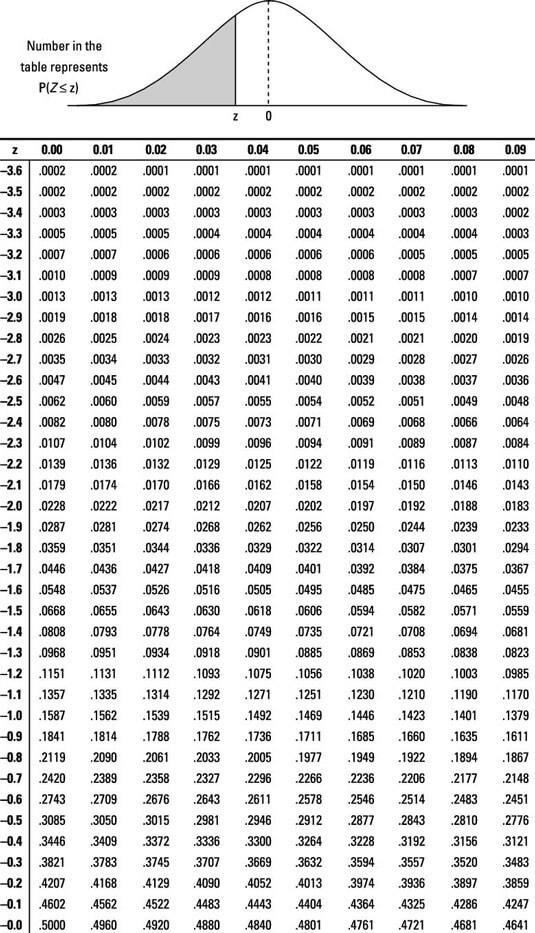
The light blue area represents the 95% probability of an outcome happening, and the dark blue represents the remaining 5%.
The p-value (probability-value) is the indicator if an outcome would happen or not, on the 95% or the 5% probability.
You don’t have to calculate the p-value for the probability. There is a table given already, and this is for the z-score (learned in lesson 1.2):
Additional explanation on p-value
Additional examples of T-Test
Groups Do: Forming a Null Hypothesis
Let’s open up the file(s) in the 01-Par_Null_Hypothesis folder to get started.
The whole goal of this activity is if you can verbalize your intent, or your hypothesis, in clear statements so that people can follow what you’re trying to prove or disprove within your test.
At work, we can have statements like:
- Did we provide enough support for indie video game developers?
- Ref: https://www.bloomberg.com/news/newsletters/2021-07-02/sony-draws-the-ire-of-indie-video-game-makers
- We are expected to frame the success metrics of what it means to provide adequate support for our publishers.
Convert the following questions into a hypothesis and a null hypothesis:
- Does dark chocolate affect arterial function in healthy individuals?
- Assume that we are referring to 30g of dark chocolate over a one-year period.
- Does coffee have anti-aging properties?
- Assume that the average dosage for consuming coffee daily is at 400mg, the average size of a mug.
T-Test
Let’s open up the file(s) in the 02-Ins_T-Test folder to get started.
A t-test is a statistical test to compare the means of 2 groups of data.
Independent (unpaired) samples / two-sample t-test
Let’s use the previous example of a electric car company. You want to know if red cars sell better than white cars.
We would compare the mean sales of red cars and white cars and determine if there is a statistically significant difference between them.
- H0: μred = μwhite
- where μred represents the population mean sales of red cars and μwhite represents the population mean sales of white cars.
- The null hypothesis would be that there is no difference in the mean sales of red cars and white cars.
- Ha: μred > μwhite
- The alternative hypothesis would be that the mean sales of red cars are greater than the mean sales of white cars.
Paired Test / One-sample test
You are still comparing two groups of data, but you’re sampling the same population of data twice.
Suppose a company wants to test the effectiveness of a new training program for its employees. To do so, they randomly select 20 employees and give them the training program. Before and after the training, each employee’s productivity is measured and recorded. The company wants to determine if the training program has had a significant effect on employee productivity.
In this case, a paired t-test would be appropriate because we have two sets of data (before and after productivity) from the same group of individuals (the 20 employees). The null hypothesis would be that there is no significant difference in productivity before and after the training program, and the alternative hypothesis would be that there is a significant difference in productivity.
- H0: μafter – μbefore = 0
- Ha: μafter – μbefore ≠ 0 (We don’t know if it is going to be a positive or negative impact.)
- Where μbefore and μafter represent the population means of productivity before and after the training program, respectively.
Notes
- You don’t have to memorize the mathematical formula. Both Excel and Pandas have inbuilt functions for us to use.
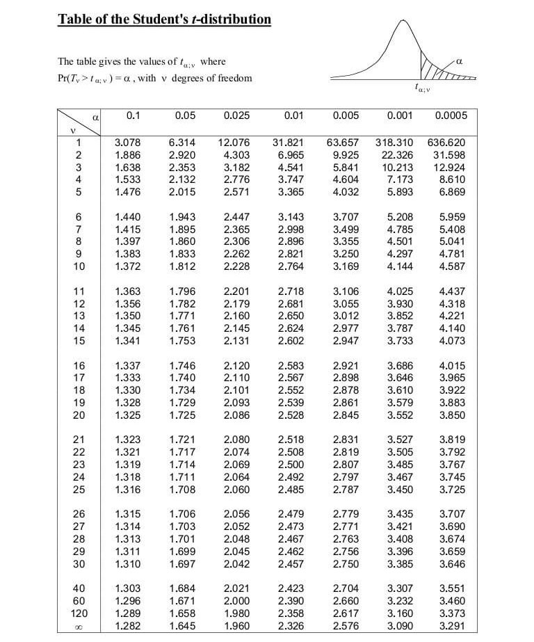
p-value table for t-test:
Additional References
Students Do: T-Test
Let’s open up the file in the 03-Stu_Stranger_Heights_T-Test folder to get started.
ANOVA: [AN]alysis [O]f [VA]riance
Let’s open up the file(s) in the 04-Ins_ANOVA folder to get started.
So far, we have been comparing and contrasting between 2 groups. ANOVA is able to test and compare the means of multiple groups.
- H0: Assumes there is no difference betwen the tested groups.
- Ha: Assumes a relationship between the tested groups.
Students Do: ANOVA
Let’s open up the file(s) in the 05-Stu_ANOVA folder to get started.
Chi Square
Let’s open up the file(s) in the 06-Ins_Chi_Square folder to get started.
What is it used for?
When you collect data, is the variation in your data due to chance or is it due to one of the variables you’re testing?
You are comparing observed values vs expected values in this test.
- H0: There is no significant difference between the observed and expected frequencies.
- Ha: There is a significant difference between the observed and expected frequencies.
Supposed you’re flipping a coin 100 times.
- In your 1st try, you got probably 65 heads vs 35 tails. That is your observation.
- However, we are expecting both 50 heads vs 50 tails.
- The whole point of this test is to reject or accept the null hypothesis. Is there a significant difference between the observed and expected frequencies?
What is degrees of freedom (df)?
It refers to the number of outcomes in a sample that are free to vary, minus 1.
- They are independent of each other.
- They contribute to the estimation of a population parameter.
They are important because they affect the distribution of certain statistical tests, such as the t-test.
In general, as the degrees of freedom increase, the distribution of the test statistic approaches a normal distribution, which helps us to infer more accurately.
- Degrees of freedom in independent samples: df = n1 + n2 – 2
- where n1 and n2 are the sample sizes of the two groups being compared.
- Degrees of freedom in dependent (paired) samples: df = n – 1
- where n is the number of pairs of observations in the sample.
Example of Degrees of Freedom
Let’s say we have a data sample consisting of 5 positive integers. Let’s also assume that the average of these 5 numbers is 6. If 4 items within the data set are {3, 8, 5, 4}, then the fifth number must be 10 to equal the average value of 6. The first 4 numbers can be chosen at random, thus, the degree of freedom is 4.
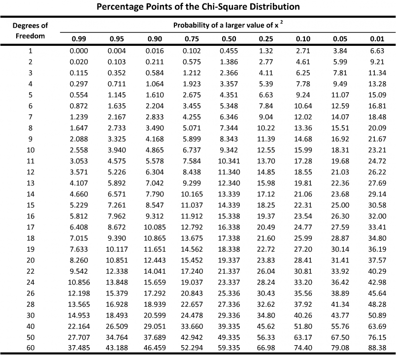
p-value table from chi-square values