
Supervised learning is where you know the outcomes or labels of what you want to predict, and you have a history or training of data that has the outcomes or labels so that you can identify the patterns from.
We are extrapolating to the future by using the past, and this forms the basis of supervised learning.
Linear Regression
Let’s open up the file(s) in the 01-Ins_Linear_Regression folder to get started.
Linear regression is the basic foundational block for other machine learning algorithm such as neural networks and deep learning.
For example, we have a function called make_regression from the sklearn.datasets library:
- sk-learn stands for scikit-learn. This is the Python library we’ll be using for the majority of this course.
- make_regression generates a random regression problem as an example:
- n_samples: Number of data points
- n_features: Number of data properties to train or predict from.
- random_state: An integer seed to replicate the example if needed.
- noise: Standard deviation applied to the output
- bias: computed value as the distance between the average prediction and true value.
This diagram should help in defining bias:
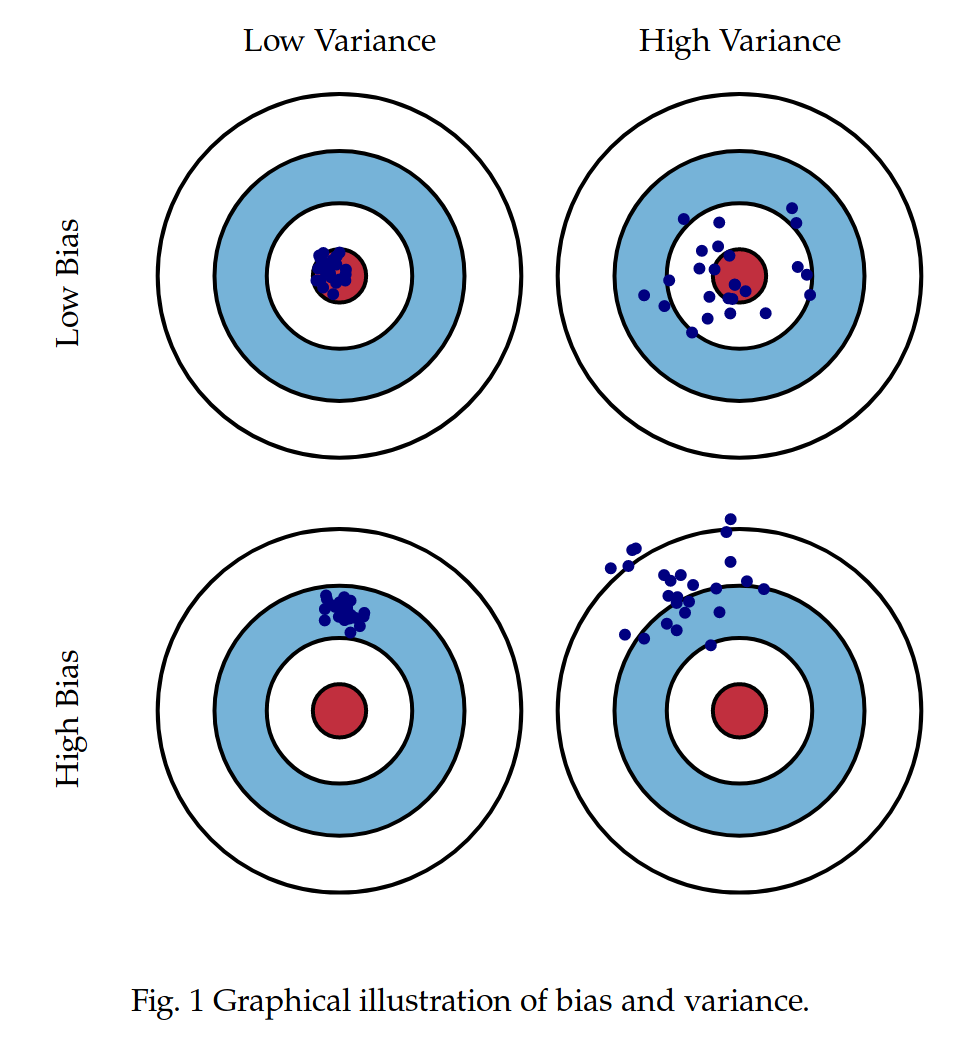
- Bullseye is the goal.
- Bias strays the aiming of your bow.
- Variance is the slight movements from your aim (your arms were tired) that results in hitting different spots around the same region.
This linear graph is to simulate a probable scenario. For example:
- We understand that the larger the house, the more expensive it is. (Let’s ignore the other factors like traffic and environment.)
- As square feet increases, we expect the home price to escalate in a linear fashion.
- It is unlikely that the home price relates to square feet in a sine curve. That would mean that at certain square feets, it will mean lower prices as indicated by the sine curve.
- But a log curve is possible, since materials’ price can sharply rise at a certain volume.
You might be planning for an apartment, and you’re looking at 1000 square feet. The linear line helps you to predict the price of the home based on other home prices indicated. That’s how linear regression and basic machine learning works in general.
Mathematical Formula
It’s going back to high school, but:y = mx + b
yis the output responsexis the input feature (we have one feature, remember? Square fit is the feature for our example.)bis the y-axis intercept.mis the gradient, or weight coefficient.
Quantifying Regression
This just means how do we prove if our model works? How do we quantify accuracy?
As we use linear regression as our foundational study material, realize that what you learned here is going to be applied to other models as well.
To quantify accuracy, we use common scoring metrics such as:
- R-Squared (R2)
- Mean Squared Error (MSE)
What I’m going to teach you are some of the fundamentals of R2 and MSE to understand how we derived accuracy, but to find out more on the mathematical derivation, look at the links below:
- R2 or coefficient of determination
- MSE (I don’t have a good math video tutorial at the moment, so you could suggest, and I’ll put it up here.)
R2 Concept
We use the margin of errors to depict the accuracy of a model. Consider this graph:
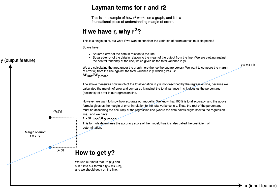
We’re trying to measure the accuracy of our model by using the margin of errors. Thus:
- Having the same input (x1), the predicted data would feature on the line, and we have the actual results as (x1,y1).
- The margin of error,
r, would bey1 - ysince there is a difference between the 2 output values. - Squaring them eliminates negatives (high school math), and we get an area on the graph.
- We can’t base our accuracy on a single margin of error. Thus, since all points have their margin of errors, we add them all up to get the Squared-Error of the line (SEline).
- But the
SElinedoesn’t allow us to compare with anything. So, we calculate the total variation inyto quantify how the margin of error against the total variance of y. - By division,
SEline/SEy-mean, we get the amount of error in relation to the total variance of y. But this describes the error percentage. How about the accuracy? - Accuracy is described by 100%, or 1 if we’re dealing with decimals. Thus,
1 - SEline/SEy-meanwill give us an accuracy score, and it’s often described as the coefficient of determination.
Beyond this will be out of our scope for math.
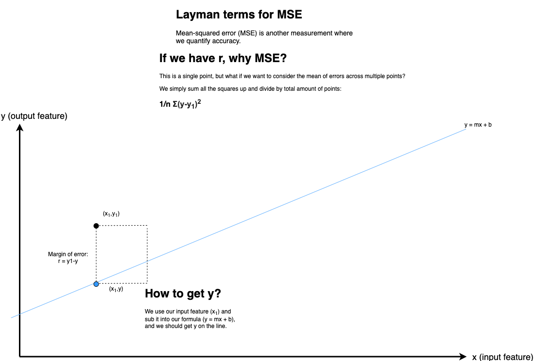
MSE Concept
Using the same concept for calculating margin of error for r2, we simply sum the squared margin of error and divide it by the total number of points:
Summary
R2value should be as close to 1 for accuracy.MSEscore should be close to 0 for accuracy.
Students Do: Predict Sales with Linear Regression
Let’s open up the file(s) in the 02-Stu_Predicting_Sales folder to get started.
Make Predictions with Logistic Regression
Let’s open up the file(s) in the 03-Ins_Logistic_Regression folder to get started.
Logistic regression is about predicting binary outcomes and the probability of it.
Train-Validate-Test
In ML, if we have a dataset, we would split the data into the following portions:
- Training Data
- This is the set of data that we will prepare our model on, by understanding the trends and features needed to meet our outcome.
- Validation Data
- We will do a preliminary prediction on this data and validate its results to have an estimated accuracy.
- Test Data
- This dataset is untouched, and it is only used for the final evaluation of the model.
How do we proportion our data into train, validation, and test?
We ensure that the test dataset is statistically significant to the rest of the dataset, and thus it depends on the number of samples needed.
However, we don’t want our training and validation datasets to be too small and then we can’t capture the trends within the dataset.
On a typical setting, we split training, validate and test data into:
- 80-10-10
- 70-15-15
- 60-20-20
What is ‘lbfgs’?
These are solver libraries that exist within sci-kit learn (and even Excel has solvers), where mathematical optimization can be easily attained using one of these libraries.
Different solvers are used in different settings, and they vary in terms of efficiency, methodology and accuracy.
It is out of scope, but lbfgs stands for “Large-scale Bound-constrained Optimization”.
Students Do: Predicting Diabetes
Let’s open up the file(s) in the 04-Stu_Predicting_Diabetes folder to get started.
Confusion Matrix & Classification Report
Let’s open up the file(s) in the 05-Ins_Classification_Models folder to get started.
Precision measure The extend of error caused by False Positives (FPs) whereas recall measures the extend of error caused by False Negatives (FNs).
We can infer that from their mathematical calculations:
- Precision = TP/(TP + FP)
- where we are including only the FP counts
- Recall = TP / (TP + FN)
- where we are including only the FN counts
This is very important based on business context, for example:
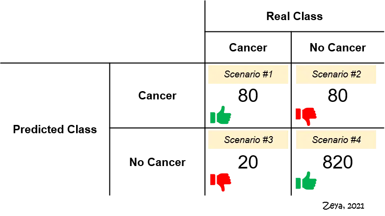
In this context, would you prefer your model to bias towards FPs or FNs?
- Scenario #2 represents FPs. Of 900 patents who really do not have cancer, the model says 80 of them do. These 80 patents will probably undergo expensive and unnecessary treatments at the expense of their well-being.
- Scenario #3 represents FNs. Of 100 patients who really have cancer, the model says 20 of them don’t. These 20 patients would go undiagnosed and fail to receive proper treatment.
*Except taken from https://towardsdatascience.com/essential-things-you-need-to-know-about-f1-score-dbd973bf1a3
Recall and precision are inversely proportional and mutually exclusive, because it is categorizing the errors into 2 distinct buckets.
How can we balance the 2 scores?
The answer is the F1-score, where F1 is the harmonic mean between the precision and recall scores.
F1-score = 2/((1/Precision) + 1/Recall))
F1 score ranges between 0 and 1, where 1 is the best.
Students Do: Classifying Social Media Influencers
Let’s open up the file(s) in the 06-Stu_Classification_Models folder to get started.
