As usual, today’s lesson is an introduction to the core concepts of neural networks. A lot less activity, but a lot more information.
Introduction to Neural Networks
Basically, neural nets were inspired by how our brains function:
- The neuron’s axos is what it uses to send signals to other neurons.
- Denrites receive information from the cell body.
- Synapses are sensors that receive signals from other neurons.
This is how our brains work:
- Brain sees an image through your eyes.
- Your brain recognizes fur, pointy ears, whiskers.
- Your brain then acknowledged that it is a cat (I know there are other things that identify a cat but let’s keep our example simple).
Likewise, we mimic the overall behavior in our code to do the same thing:
- We scan a cat image into a computer.
- The computer notices distinct vectors in on an image. Perhaps it identified fur, pointy ears, and whiskers like a humans do.
- But unlike a human, computers are only good with numbers. So if it identifies fur, it means True or 1. Then pointy ears triggers another 1, and whiskers triggers another 1. If it doesn’t notice anything, it means False or 0.
- If all three parameters are 1, we could have a function that says if all 3 parameters are 1, it is a cat and we output as True. If not, False.
- The entire system of taking inputs, and determining an output, as a single unit or entity, is called a perceptron. In-between, we have models or step-functions (activation function) to determine a result.
Of course, the example I give is simple. But if you want to classify if a skin imagery is cancerous or not, you have more than 100 million parameters to determine.
Perceptron
Actually, we are using perceptrons without realizing it:
- Logical operators
- AND, means all inputs must be True(1) to output True(1). Otherwise, False(0).
- OR, means if any of the input is True(1), output True(1). Otherwise, False(0).
Then, what is a neural network?
Layers of neurons (perceptrons) connected together to form decisions or classification of results.
Why use log regression rather simple True or False?
Because True or False gives us no room to correct and train our systems. It’s either 100% correct or 0%. The highest value of a log is 1, and the lowest is 0 (remember your high school math?), and in-between are all decimals. If we know how close are we to True (1) or False (0) through decimals, we can correct models to achieve a better result.
Backpropagation
We feed errors rates into a system, then tweak our algorithms or parameters to improve accuracy. Intuitively, when you come to me to correct code, I always break it down and see what kind of errors took place. I fix an error at a time.
Similarly, this process works in deep learning. The difference is computers are mitigating errors on a larger scale.
Tensorflow Playground
Tensorflow is what we use to for machine learning purposes. It’s a library developed by Google for all sorts of data science projects, especially neural networks.
Goggle has developed a playground for us to get acquainted with Tensorflow here: Tensorflow Playground
When you visit the playground, you can see a dashboard with lots of control and parameters. Let’s break it down somewhat:
- The top bar is a generic control panel for training.
- Play button when your formula starts training.
- Epoch is the time transpired that the model has been working.
- Time to train a model is actually a pivotal part of ML. Of course, this is a playground, and so it’s supposed to be quick, but I’ve heard cases where training data took months.
- Learning rate is a numerical parameter which allows the algorithm to adjust itself, or in other words, to reduce the errors. Basically, it’s adjusting the weight in a linear equation.
- Your school slides give an example of gradient descent, which is where the algorithm uses itself to adjust the classifier into its optimal state.
- Activation function is a mathematical function which is applied to incoming data to define an output. Usually, the outputs are binary, either True or False, Yes or No. It can get more complicated than this but we’ll rest our case here:
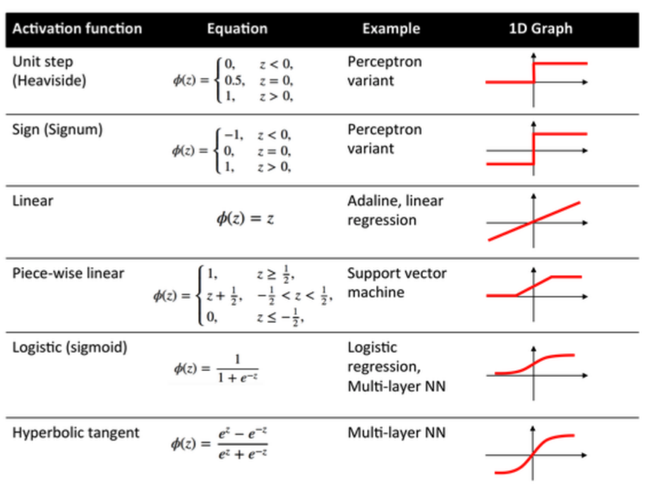
- Your school slides give a good overview of the different types of activation function that is commonly available.
- Regularization and Regularization rate is to prevent overfitting.
- L1 is called Lasso Regression.
- L2 is called Ridge Regression.
- The side bar on the left manages the data parameters.
- They don’t tell us what kind of data this is, so we assume this data as random coordinates in a bi-dimensonal scale.
- Features are the dimensions you want to define in your data set. Example. supposed you want to identify cats and dogs by 2 features, height and weight.
- Hidden Layers are the set of rules you want to define to classify the data.
- Imagine the blue dots are cats and the orange dots are dogs. This data is collected in both X1 and X2 as weight and height.
- Notice that each neuron node is a singular line? It’s binary classifcation, where one neuron determine disect the graph horizontally, while the rest disect it with slants.
- The default activation function here is hyperbolic tangent. Looking at the graph above, you have three distinct values, -1, 0, and 1. The white region denotes 0, while -1 denotes orange and 1 denotes blue. Zero is the boundary where you want to separate between cats and dogs.
- Why 2 hidden layers? If we remove the second layer, the output would show a “triangular shaped” output. That’s because we use lines to draw, and the second layer is to smoothen the edges out for a better error approximation.
- Output is self-explantory. You want to have a visualization of how you’re classifying your data.
What are you looking for in this playground?
Comparisons between different activation functions and how fast it can train your data properly.
You’ll start to see how many weak learners (algorithms & models) are ensembled to create an accurate output. Neural networks is simply a network of multi-layered weak learners that will help to classify or perform calculations towards accuracy.
One of the obvious disadvantages of deep learning is it takes a lot of processing time and compute power to get accuracy. Unless your organization has a lot of money to spend and the value far outweighs the cost, it is unlikely that you’ll see use of too much deep learning.
Installing Tensorflow
- Activate your dev env in conda:
conda activate dev - Install the tensorflow lib:
pip install tensorflow- You can include the installation within your Jupyter notebook with:
!pip install tensorflow
- You can include the installation within your Jupyter notebook with:
Students Do: Working Through the Logistics
Let’s open up the file(s) in the 01-Stu_WorkThroughLogistics folder to get started.
Why logistic regression/classification is a precursor to deep learning?
That’s because logistic algorithms allow elasticity, where the model can use to improve its accuracy.
If your activation function is only 1 or 0, True or False, it can be impossible to use deep learning to predict in certain contexts.
Setup Google Colab
Every Google account that you sign up for (in many cases, your gmail), comes with access to Google Colab.
What is Google Colab?
The main purpose of Google Colab is to run your machine learning (ML) algorithms in the cloud.
Why run ML in the cloud?
Short answer: Your local machine cannot handle the load for many real-world applications.
Long answer: Running an ML model within the cloud allows scalability and maintainability of your solution. If you need more, then ramp up the amount of compute units.
However, it comes with a price tag. Sure, they say it is free to use, but you would have to pay if you use up more resources than is allowed.
How to setup Google Colab?
Ref: https://colab.research.google.com/notebooks/welcome.ipynb
Log into your Google account first and then access the above link.
Google Colab requires you to use Google drive to host your Jupyter Notebooks.
- Take note that Google Drive has its own cost if you go over the free 15GB limit!
Connecting Google Collab With Your GDrive
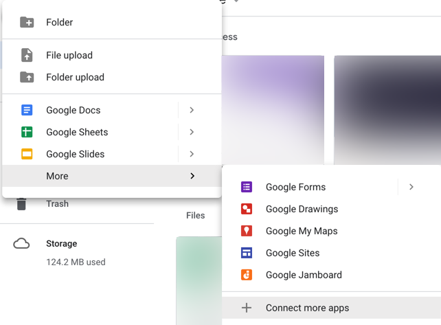
1. Go to your gDrive and look for the “More” tab as shown:
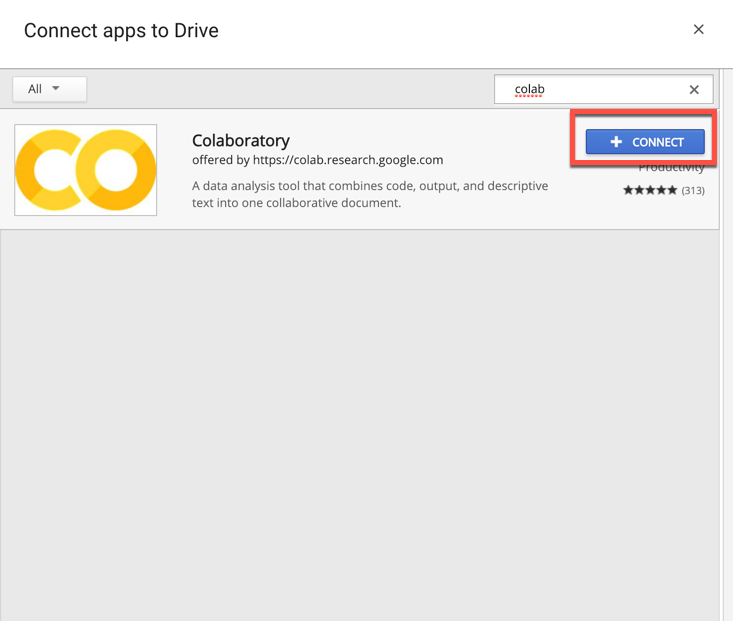
2. Search for “colab” so that you can see the Colaboratory app as shown:
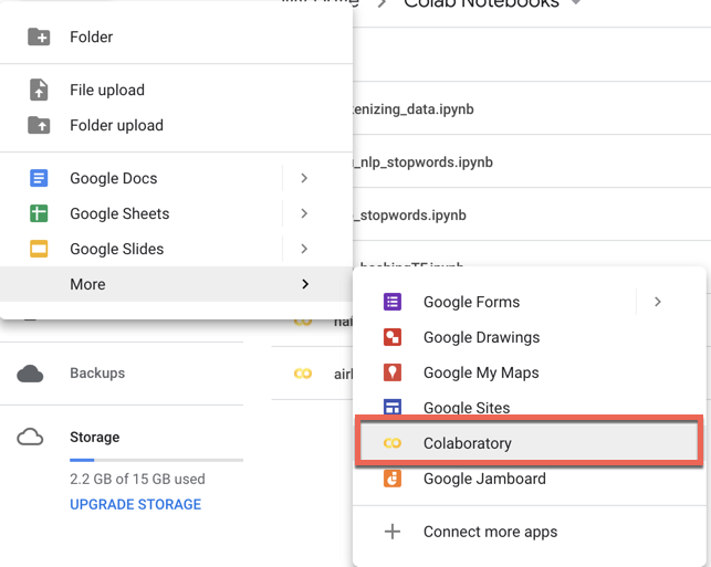
3. If you have done so, it will create the Jupyter notebook within the system:
Pro Tip:
We usually deploy with Github rather than gDrive, because there is version control. It is not covered in the course, but something you might want to explore.
Work Through a Neural Network Workflow
Let’s open up the file(s) in the 02-Ins_WorkThroughNN folder to get started.
Students Do: BYONNM—Build Your Own Neural Network Model
Let’s open up the file(s) in the 03-Stu_BYONNM folder to get started.

